41. A Lake Model of Employment#
41.1. Outline#
In addition to what’s in Anaconda, this lecture will need the following libraries:
import numpy as np
import matplotlib.pyplot as plt
41.2. The Lake model#
This model is sometimes called the lake model because there are two pools of workers:
those who are currently employed.
those who are currently unemployed but are seeking employment.
The “flows” between the two lakes are as follows:
workers exit the labor market at rate
new workers enter the labor market at rate
employed workers separate from their jobs at rate
unemployed workers find jobs at rate
The graph below illustrates the lake model.
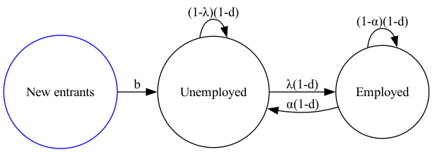
Fig. 41.1 An illustration of the lake model#
41.3. Dynamics#
Let
The total population of workers is
The number of unemployed and employed workers thus evolves according to:
We can arrange (41.1) as a linear system of equations in matrix form
Suppose at
Then,
Thus the long-run outcomes of this system may depend on the initial condition
We are interested in how
What long-run unemployment rate and employment rate should we expect?
Do long-run outcomes depend on the initial values
41.3.1. Visualising the long-run outcomes#
Let us first plot the time series of unemployment
class LakeModel:
    """
    Solves the lake model and computes dynamics of the unemployment stocks and
    rates.

    Parameters:
    ------------
    λ : scalar
        The job finding rate for currently unemployed workers
    α : scalar
        The dismissal rate for currently employed workers
    b : scalar
        Entry rate into the labor force
    d : scalar
        Exit rate from the labor force

    """
    def __init__(self, λ=0.1, α=0.013, b=0.0124, d=0.00822):
        self.λ, self.α, self.b, self.d = λ, α, b, d

        λ, α, b, d = self.λ, self.α, self.b, self.d
        self.g = b - d
        g = self.g

        self.A = np.array([[(1-d)*(1-λ) + b,   α*(1-d) + b],
                           [        (1-d)*λ,   (1-α)*(1-d)]])


        self.ū = (1 + g - (1 - d) * (1 - α)) / (1 + g - (1 - d) * (1 - α) + (1 - d) * λ)
        self.ē = 1 - self.ū


    def simulate_path(self, x0, T=1000):
        """
        Simulates the sequence of employment and unemployment

        Parameters
        ----------
        x0 : array
            Contains initial values (u0,e0)
        T : int
            Number of periods to simulate

        Returns
        ----------
        x : iterator
            Contains sequence of employment and unemployment rates

        """
        x0 = np.atleast_1d(x0)  # Recast as array just in case
        x_ts= np.zeros((2, T))
        x_ts[:, 0] = x0
        for t in range(1, T):
            x_ts[:, t] = self.A @ x_ts[:, t-1]
        return x_ts
lm = LakeModel()
e_0 = 0.92          # Initial employment
u_0 = 1 - e_0       # Initial unemployment, given initial n_0 = 1

lm = LakeModel()
T = 100         # Simulation length

x_0 = (u_0, e_0)
x_path = lm.simulate_path(x_0, T)

fig, axes = plt.subplots(3, 1, figsize=(10, 8))


axes[0].plot(x_path[0, :], lw=2)
axes[0].set_title('Unemployment')

axes[1].plot(x_path[1, :], lw=2)
axes[1].set_title('Employment')

axes[2].plot(x_path.sum(0), lw=2)
axes[2].set_title('Labor force')

for ax in axes:
    ax.grid()

plt.tight_layout()
plt.show()
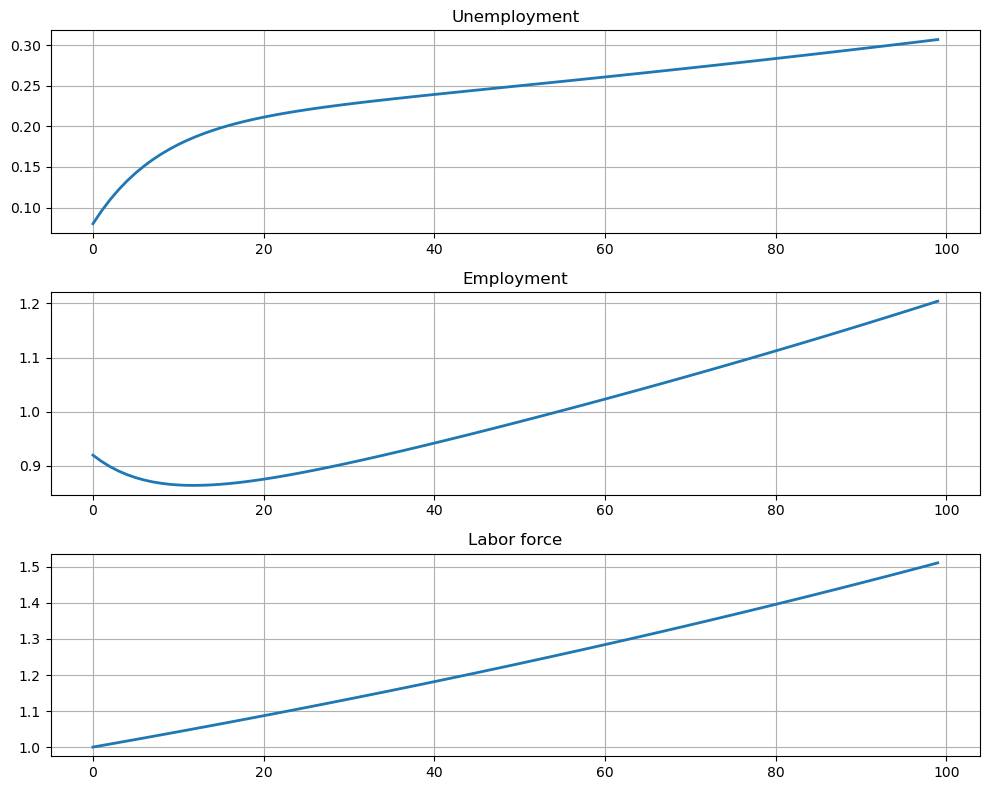
Not surprisingly, we observe that labor force
This coincides with the fact there is only one inflow source (new entrants pool) to unemployment and employment pools.
The inflow and outflow of labor market system is determined by constant exit rate and entry rate of labor market in the long run.
In detail, let
Observe that
Hence, the growth rate of
Moreover, the times series of unemployment and employment seems to grow at some stable rates in the long run.
41.3.2. The application of Perron-Frobenius theorem#
Since by intuition if we consider unemployment pool and employment pool as a closed system, the growth should be similar to the labor force.
We next ask whether the long-run growth rates of
The answer will be clearer if we appeal to Perron-Frobenius theorem.
The importance of the Perron-Frobenius theorem stems from the fact that firstly in the real world most matrices we encounter are nonnegative matrices.
Secondly, many important models are simply linear iterative models that
begin with an initial condition
This theorem helps characterise the dominant eigenvalue
41.3.2.1. Dominant eigenvector#
We now illustrate the power of the Perron-Frobenius theorem by showing how it helps us to analyze the lake model.
Since
the spectral radius
any other eigenvalue
there exist unique and everywhere positive right eigenvector
if further
The last statement implies that the magnitude of
Therefore, the magnitude
Recall that the spectral radius is bounded by column sums: for
Note that
Denote
The Perron-Frobenius implies that there is a unique positive eigenvector
Since
This dominant eigenvector plays an important role in determining long-run outcomes as illustrated below.
def plot_time_paths(lm, x0=None, T=1000, ax=None):
        """
        Plots the simulated time series.

        Parameters
        ----------
        lm : class
            Lake Model
        x0 : array
            Contains some different initial values.
        T : int
            Number of periods to simulate

        """


        if x0 is None:
            x0 = np.array([[5.0, 0.1]])

        ū, ē = lm.ū, lm.ē

        x0 = np.atleast_2d(x0)

        if ax is None:
            fig, ax = plt.subplots(figsize=(10, 8))
            # Plot line D
            s = 10
            ax.plot([0, s * ū], [0, s * ē], "k--", lw=1, label='set $D$')

        # Set the axes through the origin
        for spine in ["left", "bottom"]:
            ax.spines[spine].set_position("zero")
        for spine in ["right", "top"]:
            ax.spines[spine].set_color("none")

        ax.set_xlim(-2, 6)
        ax.set_ylim(-2, 6)
        ax.set_xlabel("unemployed workforce")
        ax.set_ylabel("employed workforce")
        ax.set_xticks((0, 6))
        ax.set_yticks((0, 6))


        # Plot time series
        for x in x0:
            x_ts = lm.simulate_path(x0=x)

            ax.scatter(x_ts[0, :], x_ts[1, :], s=4,)

            u0, e0 = x
            ax.plot([u0], [e0], "ko", ms=2, alpha=0.6)
            ax.annotate(f'$x_0 = ({u0},{e0})$',
                        xy=(u0, e0),
                        xycoords="data",
                        xytext=(0, 20),
                        textcoords="offset points",
                        arrowprops=dict(arrowstyle = "->"))

        ax.plot([ū], [ē], "ko", ms=4, alpha=0.6)
        ax.annotate(r'$\bar{x}$',
                xy=(ū, ē),
                xycoords="data",
                xytext=(20, -20),
                textcoords="offset points",
                arrowprops=dict(arrowstyle = "->"))

        if ax is None:
            plt.show()
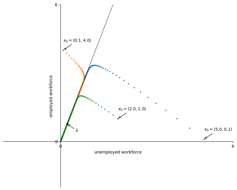
lm = LakeModel(α=0.01, λ=0.1, d=0.02, b=0.025)
x0 = ((5.0, 0.1), (0.1, 4.0), (2.0, 1.0))
plot_time_paths(lm, x0=x0)
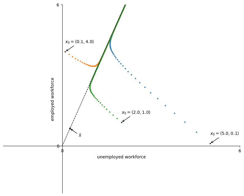
Since
This set
The graph illustrates that for two distinct initial conditions
This suggests that all such sequences share strong similarities in the long run, determined by the dominant eigenvector
41.3.2.2. Negative growth rate#
In the example illustrated above we considered parameters such that overall growth rate of the labor force
Suppose now we are faced with a situation where the
This means that
What would the behavior of the iterative sequence
This is visualised below.
lm = LakeModel(α=0.01, λ=0.1, d=0.025, b=0.02)
plot_time_paths(lm, x0=x0)
Thus, while the sequence of iterates still moves towards the dominant eigenvector
This is a result of the fact that
This leads us to the next result.
41.3.3. Properties#
Since the column sums of
Perron-Frobenius theory implies that
As a result, for any
as
We see that the growth of
Moreover, the long-run unemployment and employment are steady fractions of
The latter implies that
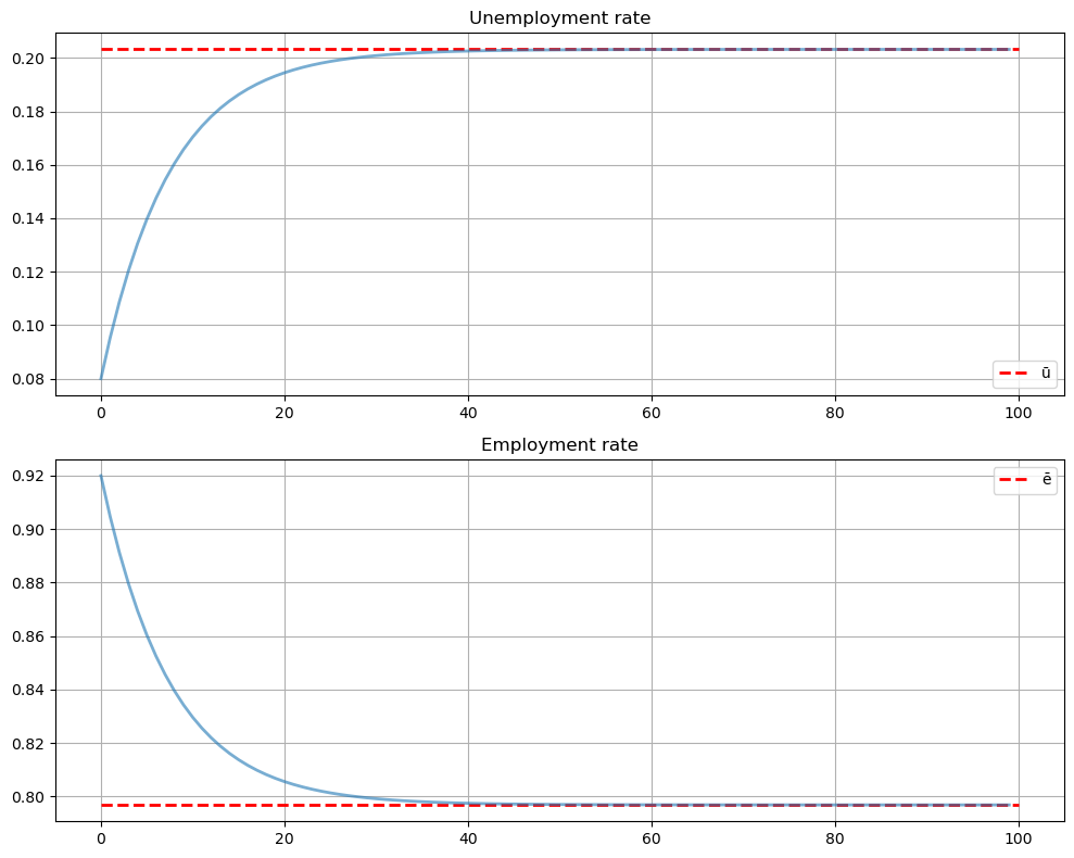
In detail, we have the unemployment rates and employment rates:
To illustrate the dynamics of the rates, let
The dynamics of the rates follow
Observe that the column sums of
One can check that
Moreover,
This is illustrated below.
lm = LakeModel()
e_0 = 0.92          # Initial employment
u_0 = 1 - e_0       # Initial unemployment, given initial n_0 = 1

lm = LakeModel()
T = 100         # Simulation length

x_0 = (u_0, e_0)

x_path = lm.simulate_path(x_0, T)

rate_path = x_path / x_path.sum(0)

fig, axes = plt.subplots(2, 1, figsize=(10, 8))

# Plot steady ū and ē
axes[0].hlines(lm.ū, 0, T, 'r', '--', lw=2, label='ū')
axes[1].hlines(lm.ē, 0, T, 'r', '--', lw=2, label='ē')

titles = ['Unemployment rate', 'Employment rate']
locations = ['lower right', 'upper right']

# Plot unemployment rate and employment rate
for i, ax in enumerate(axes):
    ax.plot(rate_path[i, :], lw=2, alpha=0.6)
    ax.set_title(titles[i])
    ax.grid()
    ax.legend(loc=locations[i])


plt.tight_layout()
plt.show()
To provide more intuition for convergence, we further explain the convergence below without the Perron-Frobenius theorem.
Suppose that
Let
The dynamics of the rates follow
Consider
Then, we have
Hence, we obtain
Since
Therefore, the convergence follows
Since the column sums of
In this case,
41.4. Exercise#
Exercise 41.1 (Evolution of unemployment and employment rate)
How do the long-run unemployment rate and employment rate evolve if there is an increase in the separation rate
Is the result compatible with your intuition?
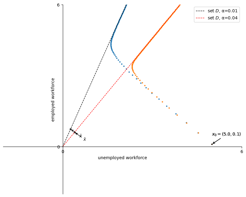
Plot the graph to illustrate how the line
Solution to Exercise 41.1 (Evolution of unemployment and employment rate)
Eq. (41.3) implies that the long-run unemployment rate will increase, and the employment rate will decrease
if
Suppose first that
The below graph illustrates that the line
fig, ax = plt.subplots(figsize=(10, 8))

lm = LakeModel(α=0.01, λ=0.1, d=0.02, b=0.025)
plot_time_paths(lm, ax=ax)
s=10
ax.plot([0, s * lm.ū], [0, s * lm.ē], "k--", lw=1, label='set $D$, α=0.01')

lm = LakeModel(α=0.04, λ=0.1, d=0.02, b=0.025)
plot_time_paths(lm, ax=ax)
ax.plot([0, s * lm.ū], [0, s * lm.ē], "r--", lw=1, label='set $D$, α=0.04')

ax.legend(loc='best')
plt.show()